Researchers
Leda Sox1*, Vincent B. Wickwar1, Tao Yuan1, Neal R. Criddle1
- Center of Atmospheric and Space Science
Abstract
We present an unprecedented comparison of temperature measurements from the Rayleigh-scatter (RS) and sodium (Na) lidar techniques. The extension of the RS technique into the lower thermosphere that has been achieved by the group at Utah State University (USU), enables simultaneous, common-volume measurements by the two lidar systems hosted in the Atmospheric Lidar Observatory at USU. The two lidars’ nightly averaged temperatures from 80-105 km, based on 19 nights of observations, are explored.
Introduction
Lidar systems remain the most advantageous method for acquiring temperature measurements of the Mesosphere-Lower Thermosphere (MLT) region (~45-115km), in terms of vertical and temporal resolution. Two of the most widely used lidar techniques for MLT studies are RS and Na lidar. RS lidar systems measure elastic backscatter from neutral N2, O2, Ar, and O particles in the atmosphere. RS lidar backscatter measurements give relative density profiles, which are then used to calculate absolute temperature profiles [1, 2]. Na lidar measures laser-induced resonant fluorescence from the mesospheric Na layer, which forms in the 80-105 km region of the atmosphere due to meteor ablation. With proper design, Na lidars can measure thermal broadening and Doppler shifts of the laser-induced fluorescent Na spectrum. From this, Na density, temperature, and winds can be deduced [3]. Two climatological studies have compared results from the RS and Na lidar techniques using composite year averages from lidar sites spread around the globe, over different observational periods [4, 5]. In Argall and Sica [4], RS temperatures were found to be 7 K cooler than Na temperatures in the altitude range of 80-95 km. Leblanc et al. [5], found RS temperatures, from 82-88 km, to be 8-14 K colder than the Na temperatures from 80-82 km and 2-6 K colder from 82-88 km. The present study aims to explore these temperature differences using RS and Na lidar measurements made simultaneously, from the same facility, and over the same observational range.
Methodology
Between summer 2014 and summer 2015, there were 19 nights, which spanned all four seasons, when the two USU lidars made simultaneous measurements in the MLT region throughout the night. This dataset is relatively small due to the different observational schedules that are employed by each group. Since the Na lidar can observe over full diurnal cycles, the Na lidar group typically conducts campaigns once a month for three to five days and nights. While the RS lidar cannot currently operate in the daytime, the RS group aims to observe every clear night throughout the year. The difference in observational schedules allows the two lidar systems’ datasets to complement each other well, but also means simultaneous measurements are infrequent unless deliberately planned. The RS system is capable of acquiring temperature profiles from 70-115 km, while the Na lidar’s temperatures can span 80-110 km. For the most part, however, the two lidar systems measurements overlapped in the 80-105 km range, since these altitude limits can change from night-to-night depending on atmospheric and instrumental conditions for the RS lidar and on the width of the sodium layer for the Na lidar. Simultaneous, nightly-averaged temperature profiles were calculated for each lidar’s dataset to avoid biases induced by atmospheric gravity waves. Each lidar’s nightly averages are at least four hours long, and the beginning and end times for both averages were set to be within two minutes of one another before data processing. The temperature profiles from each lidar, along with a profile from the MSISe00 model [6] at the USU location, were investigated for all 19 nights. Figure 1 shows four examples of these lidar comparisons. The error bars plotted with the RS and Na curves were calculated by propagating the measurement error (from photon counting) through each lidar’s respective temperature reduction process [2, 3]. A seed temperature is required for the top RS altitude in order to initiate the RS temperature reduction. These were taken from the Na lidar’s temperatures [e.g. Figure 1(d)], except on nights when the RS lidar’s temperatures went higher than the Na lidar’s [e.g. Figure 1(a), (b), and (c)]. On these nights, values from MSISe00 are used.
Results
The four temperature curves shown in Figure 1 are from each of the four seasons between summer 2014 and summer 2015. Figure 1 shows that, although the two sets of temperatures agree very well during most of the lidar campaign, differences between the two lidars’ temperature measurements are noticeable in some of the 19 nights’ observations. For example, in Figure 1(a), very large temperature differences (ΔT up to ~50 K, where ΔT=TRS-TNa) between the two lidars’ temperatures are seen above 90 km, while the geomagnetic activity was low. In Figure 1(b), the two temperature curves show the best agreement at all altitudes. Figures 1(c) and (d) exemplify the typical behavior of the whole dataset. This behavior is characterized by the RS lidar temperatures being slightly cooler (-5 K≤ΔT<0 K) at lower altitudes (80-85 km); the two temperature curves being within a few degrees (-5 K≤ΔT≤5 K) of one another in the middle of the altitude range (85-95 km); and the RS temperatures being warmer (5 K≤ΔT≤50 K), at higher altitudes (95 km and higher).
Figure 1 is representative temperature plots for nightly averages determined using the RS lidar (blue curves) and Na lidar (red curves). MSISe00 model temperatures (black curves) for each date at 6 UT and USU’s geographical coordinates, are also given. A profile from each season (summer, fall, winter, and spring) is presented: (a) 20 June 2014, (b) 26 September 2014, (c) 09 November 2014, and (d) 14 April 2015.
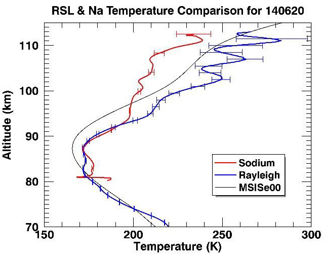
Figure 1(a)
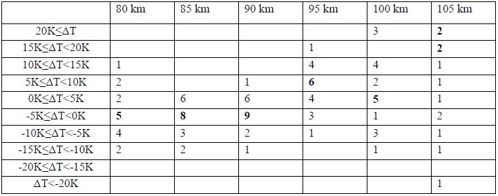
These differences at altitudes above 95 km are often statistically significant, exceeding both lidars’ error bars [e.g. Figure 1(a), (c), and (d)]. This pattern is elucidated in Table 1, which gives the number of nights that ΔT fell into a specific interval at a given height. Here, each lidar’s temperatures were averaged over 1 km intervals (e.g. 85 to 86 km, 90 to 91 km, etc.) and then used to calculate ΔT. On some nights, there is also a difference in the structure of the temperature profile at higher altitudes, where the RS temperatures show stronger and more distinct wave structure than the Na temperatures. Examples of this incongruent wave structure can be seen in Figure 1(a).
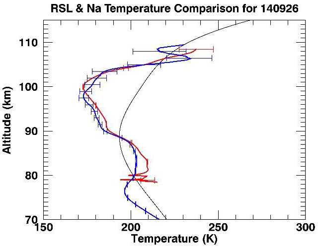
Figure 1(b)
Similar distinct structures are also observed in 6 of the 19 nights throughout the year (140620, 140723, 140912, 140913, 141029, and 141106, in YYMMDD). These wave features in the RS profiles are puzzling and cannot be explained properly at the moment. The Na lidar has showed that long lasting, large-scale temperature inversion structures exist in the mesopause region due to wave breaking [7]. However, it did not detect any of these structures at these altitudes during these nights. It would be highly difficult for such long-period inertia gravity waves to reach near and beyond 100 km due to the severe atmospheric dissipation they experience, as they slowly propagate upward.
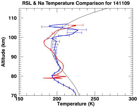
Figure 1(c)
Another interesting observation is that the nights with the best agreement between the two lidars’ temperatures, over the entire 80-105 km altitude range, are all close to the fall (140923) and spring (150320) equinoxes, which can be seen in Figure 1(b) and was also observed on 140925 and 150328. The two lidars’ temperatures agree much better with one another than they do with the MSISe00 model temperatures. For the most part, if one lidar’s temperature profile is either warmer or colder than the MSISe00 temperatures, then the other lidar’s temperatures behave the same way. There are 5 exceptions, however, throughout the year (140620, 140722, 140912, 141108, and 141109), an example of which can be seen in Figure 1(a).
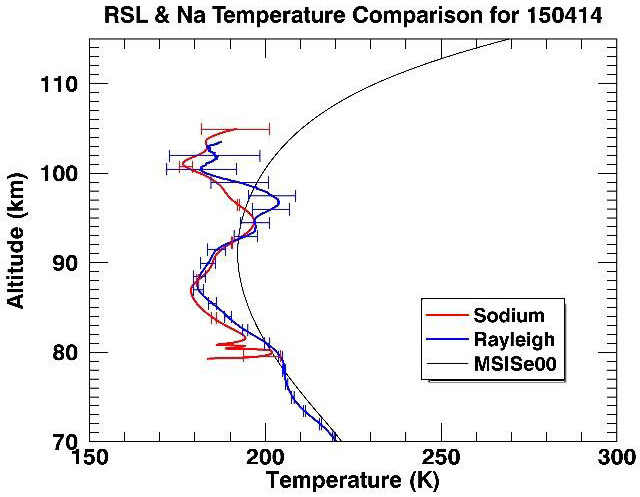
Figure 1(d)
In all of these cases, above 90 km, the Na temperatures are colder than MSISe00 temperatures, whereas the RS temperatures are warmer. Two of these nights were also nights when the RS lidar showed the strong wave structure mentioned before. While the overall structure of the lidars’ temperature profiles are roughly similar to the MSISe00 structure, there were 7 cases, mostly in the fall and winter, (140912, 140913, 140925, 140926, 141104, 141106, and 141108) where the lidars’ mesopauses were at different altitudes than the MSISe00 mesopause, as in Figure 1(b) and (c).
Conclusions
We have presented a unique comparison of simultaneous temperatures acquired by a Rayleigh- scatter lidar and a sodium resonance lidar collocated in the Atmospheric Lidar Observatory on the campus of Utah State University. The two sets of temperature data also overlap in altitude (80-105 km). Our simultaneous, common-volume RS and Na lidar measurements showed, like previous climatological comparisons in the 80-90 km region [4, 5], that the RS lidar’s temperatures were on average colder than the Na lidar’s temperatures. However, the magnitude of our differences (-5 K≤ΔT<0 K), was smaller than the previous studies’. Above 95 km, we have shown new results that were not possible in the previous studies, due to the altitude limitations of older RS systems. The results indicate that the RS temperatures are warmer than the Na temperatures in this region (5 K≤ΔT<50 K). The RS lidar temperatures also show stronger and more distinct wave activity than the Na temperatures above about 90 km, which demands more investigation in the future. The best agreement between the two techniques’ temperatures, throughout the entire 80-105 km range, occurs on the nights, albeit only three, closest to the equinoxes. The two lidar techniques typically agree with one another better than each does with the MSISe00 model. When they disagree, the RS lidar’s temperatures are typically warmer than MSISe00, while the Na lidar’s temperatures are colder. In the future, we aim to take enough simultaneous measurements with the two USU lidars to obtain good coverage throughout all months in order to further explore the day-to-day and seasonal differences between the two systems’ deduced temperatures and, especially, to explore the differences above 95 km.
Acknowledgements
The original RS lidar was initially upgraded to the much more sensitive configuration with funds from NSF, AFOSR, and USU. The system was further upgraded to bring it on line with funds provided by the Space Dynamics Laboratory Internal Research and Development program, USU, the USU Physics Department, and personal contributions. The Na lidar was supported under NSF AGS grant number 1135882. The RS and Na lidar data presented in this paper were acquired through the dedicated efforts of many USU student operators and engineers.
References
- Hauchecorne, A., and Chanin, M.-L., 1980: Density and temperature profiles obtained by lidar between 35 and 70 km, Geophys. Res. Lett.,7, 565–568, doi:10.1029/GL007i008p00565.
- Sox, L., 2016: Rayleigh-Scatter Lidar Measurements of the Mesosphere and Thermosphere and Their Connections to Sudden Stratospheric Warmings, Utah State Univ.,Logan, UT, 212pp, http://digitalcommons.usu.edu/etd/5227.
- Krueger, D. A., She, C. Y., Yuan, T., 2015: Retrieving mesopause temperature and line-of-sight wind from full-diurnal-cycle Na lidar observations, Appl. Opt., 54, 9469–9489, doi:10.1364/AO.54.009469.
- Argall, P. S., and Sica, R. J., 2007: A comparison of Rayleigh and sodium lidar temperature climatologies, Ann. Geophys., 25, 27–33, doi:10.5194/angeo-25-27-2007.
- Leblanc, T., McDermid, I. S., Keckhut, P., Hauchecorne, A., She, C. Y., Krueger, D. A., 1998: Temperature climatology of the middle atmosphere from long-term lidar measurements at middle and low latitudes, J. Geophys. Res.,103(D14), 17191–17204, doi:10.1029/98JD01347.
- Picone, J. M., Hedin, A. E., Drob, D. P., Aiken A. C., 2002: NRLMSISE-00 empirical model of the atmosphere: Statistical comparisons and scientific issues, J. Geophys. Res.,107(A12), 1468, doi:10.1029/2002JA009430.
- Yuan, T., Pautet, P.-D., Zhao, Y., Cai, X., Criddle, N. R., Taylor, M. J., Pendleton Jr., W. R., 2014: Coordinated investigation of mid-latitude upper mesospheric temperature inversion layers and the associated gravity wave forcing by Na lidar and Advanced Mesospheric Temperature Mapper in Logan, Utah, J. Geophys. Res. Atmos.,119, 3756–3769, doi:10.1002/2013JD020586.
Source
- Sox, L., Wickwar, V. B., Yuan, T., & Criddle, N. R. (2018). Comparison of rayleigh-scatter and sodium resonance lidar temperatures. EPJ Web of Conferences, 176, 03005. doi:10.1051/epjconf/201817603005