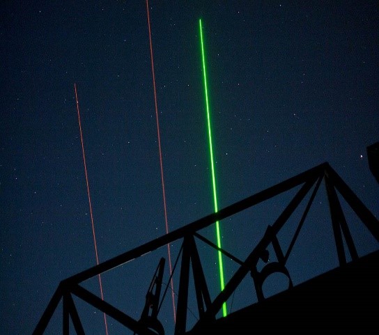
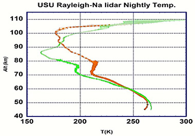
Figure 1. Simultaneous Na lidar (orange) and Rayleigh lidar (green) observations at the Atmospheric Lidar Observatory at USU (left). The nightly averaged temperatures profiles (right) observed at USU (42°N, 112°W) on two nights (Apr. 7th and July 12th) in 2016. The temperatures below 80 km (Rayleigh lidar); those above 80 km (Na lidar) (Yuan et al.).
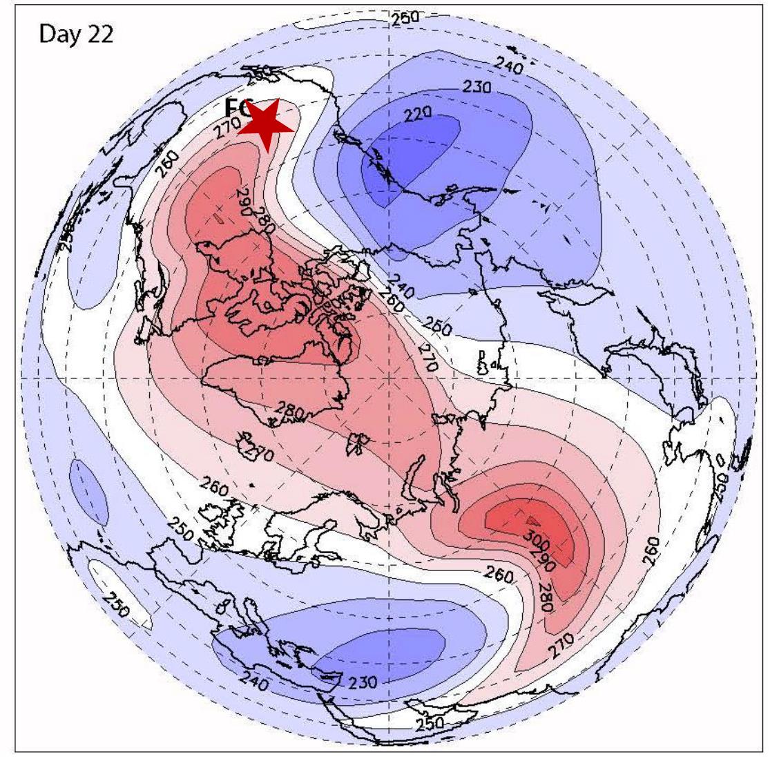
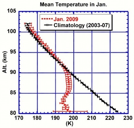
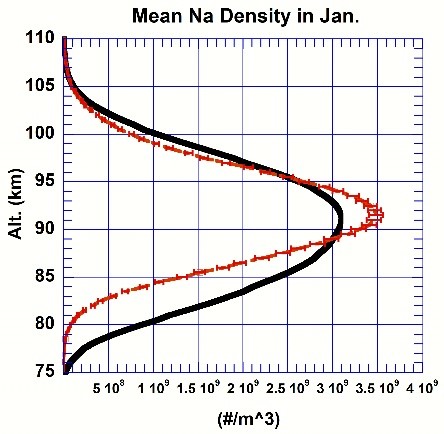
Figure 2. Longitudinal temperature distribution at midnight UT on Jan. 22th, 2009 at 40 km altitude using the specified dynamic mode WACCM simulation (left). The red star in the top left sector indicates the lidar location. Na lidar measured mean MLT temperatures between Jan.19th and Jan. 21st prior to SSW compared with climatological mean temperature profile (middle), showing cooling occurred earlier in MLT, while the Na density experienced dramatic depletion in the upper mesosphere (right) (Yuan et al.).
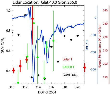
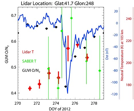
Figure 3. Time sequence of the Na lidar nightly averaged temperature at 105 km (red diamonds with error bars) during the courses of the four storms, along with the variations of Dst index (blue solid lines) and TIMED/GUVI daily observations of thermospheric column density O/N2 (black diamonds) at the lidar stations. TIMED/SABER temperatures at 105 km within the grid that covers ±5° longitude and ±5° latitude over the lidar site during the 2004 and 2012 storms are also plotted (Yuan et al., 2015).